
This post is part of a longer series on map design questions. I have not written much more recently on my work on the alternative-colors style and there is a bit of a backlog of topics that deserve some discussion. I will make a start here with the most heavy of all – the roads. In this first part i am going to explain the OSM-Carto road rendering system and analyze its issues and limitations.
The challenge of depicting roads
The without doubt most complicated part and for any OSM-Carto map style developer the most serious challange when working on OSM-Carto or one of its derivatives is the roads layers. As Paul some time ago compactly put it the roads rendering in OSM-Carto alone is more complex than many other map styles are in total. Roads (and in context of OSM-Carto roads by the way generally refers to all lines and other features along which land navigation of humans takes place – including roads for automobile navigation, paths for navigation by foot, animal or other vehicle as well as railways and traditionally also runways and taxiways on airports, which however have more recently been moved outside of the roads layer system in OSM-Carto) can be complex in their semantics, connectivity and above all in their vertical layering. Representing that in a well readable and accurate way in a map is a challenge to put it mildly.
Most simpler map styles take shortcuts in this field – which tends to show up in map in non-trivial situations. See for example the following case example:
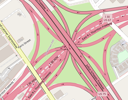
Road example in Dallas, US in OSM-Carto
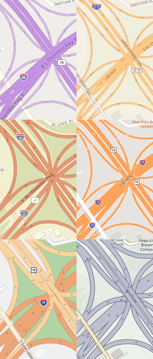
Same example in other maps: left side from top: Bing, Esri, TomTom, right side from top: Maptiler, Mapbox, Thunderforest
All maps have their flaws in roads rendering – OSM-Carto in particular with the labeling – which however is a different matter that i am not going to cover here. But beyond that it offers by far the most consistent display of the connectivity and layering of the roads in this intersection.
The way this is done in OSM-Carto i will describe in a moment – but before i want to emphasize that OSM-Carto producing a consistent rendering of how the roads are mapped in OpenStreetMap is of high importance for the quality of data in OSM. It helps ensuring that the information that is necessary for an accurate interpretation of the data is mapped and that the reality is not recorded in a distorting fashion to achieve a certain rendering result. More than in any other field of mapping in OpenStreetMap probably the rules of mapping roads have been developed in connection with how the data is used in rendering while still maintaining the principle that what is mapped and tagged represents verifiable elements of the geography and not just prescriptions how things are supposed to show up in the map. This is an accomplishment that cannot be overstated and that is important to maintain and extend in the future.
The OSM-Carto road layers
To understand the way OSM-Carto renders roads it is important to first understand how the drawing order is defined in the toolchain used by OSM-Carto (Carto and Mapnik). In decreasing priority the drawing order is defined by the following:
- The layers of the map style: Data that is rendered in the map is queried from the rendering database in the form of distinct and separate layers and is rendered in exactly the same order. The layer stack is defined in project.mml and starts with the landcover layers (at the very bottom) and ends with labels.
- The group-by parameter of the layer in question (in case it is present): The way this works is that the query of the layer is ordered primarily by one column of the results table and by specifying this as group-by parameter you tell carto/mapnik to group the features by that parameter and render them kind of like they were in separate layers.
- The attachments in MSS code. That is the
::fooselectors. Those kind of work as a method to accomplish layered drawing within a single layer. But in contrast to the group-by parameter every attachment needs to be coded explicitly, you cannot automatically base attachments creation on some attribute in the data. - The order in which the data is queried in SQL (typically through an
ORDER BYstatement) - The instances of the drawing rules in MSS code: Those are the prefix with a slash you put in front of the drawing rules. Like
a/line-width: 2; b/line-width: 4;Such rules lead to several lines being drawing, one immediately after the other, on a per-feature basis.
OSM-Carto contains exactly two layers that use the group-by feature: The tunnels and the bridges layers for the roads. Overall the roads related layers (and other layers in between) look like this (from bottom to top):
- tunnels (with
group-by layernotnull): with attachments ::casing(high zoom only),::bridges_and_tunnels_background(high zoom only),::halo(low zoom only),::fill - landuse-overlay (military landuse overlay)
- tourism-boundary (theme park and zoo outlines)
- barriers (line barriers like fences, hedges etc.)
- cliffs
- ferry-routes
- turning-circle-casing
- highway-area-casing
- roads-casing: with attachment
::casing - highway-area-fill
- roads-fill: with attachments
::halo(low zoom only),::fill - turning-circle-fill
- aerialways
- roads-low-zoom: with attachment
::halo - waterway-bridges
- bridges (with
group-by layernotnull): with attachments::casing(high zoom only),::bridges_and_tunnels_background(high zoom only),::halo(low zoom only),::fill
To better understand the terminology used – here an illustration for how the different parts of the road signature are called.
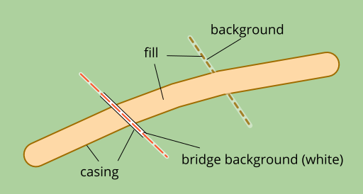
Road signature elements at high zoom levels (z18)

Road signature elements at low zoom levels (z11)
All the individual road line layers (tunnels, roads-casing, roads-fill and bridges) are ordered in SQL primarily by layernotnull (which is the layer tag with an implicit default value of zero assumed) and by z_order – which represents the hierarchy of road classes.
If we ignore most of the non-road layers for the moment and focus on the high zoom levels we have essentially the following drawing order:
- tunnels – ordered by
- layer
- casing, background, fill
- z_order (+ some other criteria in SQL)
- casings of normal non-tunnel, non-bridge roads – ordered by
- first turning circles, then polygons, then linear ways
- layer
- z_order (+ some other criteria in SQL)
- fills of normal non-tunnel, non-bridge roads – ordered by
- first polygons, then linear ways, then turning circles
- layer
- z_order (+ some other criteria in SQL)
- waterway bridges – ordered by
- layer
- bridges – ordered by
- layer
- casing, background, fill
- z_order (+ some other criteria in SQL)
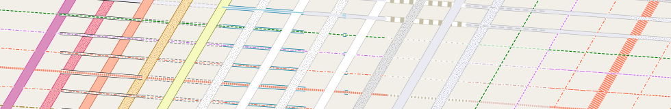
This is how this looks like visually:
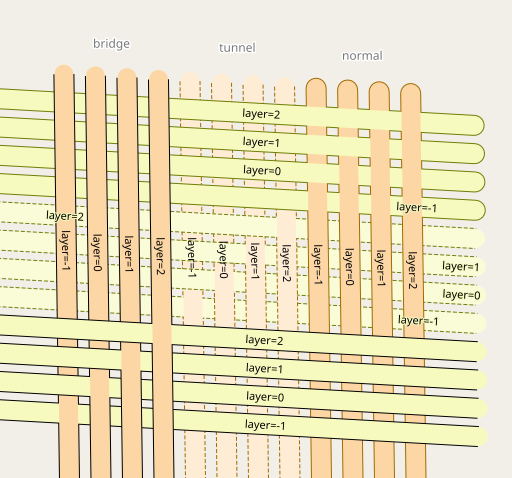
Layering of linear roads in OSM-Carto
That ordering alone however – despite its complexity – does not ensure a consistent depiction of the roads network. That also relies on the specific way the road lines are drawn. To understand this have a look at the following illustration.

Bridge drawing principles with different layers connecting
It shows self intersecting road loops as either tunnels or bridges. On the left how this is rendered when mapped as a single way. To actually represent a road crossing over above itself in form of a bridge or tunnel rather than intersecting with itself on the same level you have to split the way into two and assign different layer values.
That the two ways still visually connect where they meet at the top with their ends depends on the way they are drawn with flat line caps for the casing and round line caps for the fill. This leads – as you can see in the rightmost version – to some smaller artefacts when the bridge/tunnel way ends meet at an angle. That brings me to technical mapping rule number one that is good to consider in mapping:
Bridge or tunnel ways connecting at their ends should always have collinear segments where they meet.
The other thing that i hope this explanation shows is the meaning of the layer tag in OpenStreetMap. The wiki is fairly detailed on this but also a bit confusing. What the layer tag does is describing the relative vertical position of the physical object the feature represents, in particular a road, relative to other elements in the immediate vicinity that it is not connected with. It does not define the drawing order in the map (which depends on how exactly the map shows different features), it does not document the vertical position of a feature relative to ground level. This leads to the second technical mapping rule you can take away from this
Use the layer tag sparsely (both in the extent of where you apply it and regarding what cases you apply it in) where it is necessary to avoid ambiguities in the description of the 3d topology of what is represented by the data.
In all other cases there are other tags that will most likely better describe what you want to document – like bridge=*, tunnel=* location=underground, level=*. Or you are trying to do something you should not do (like – as a mapper – drawing the map yourself).
Limitations of this approach
Some limitations of the described system of road drawing are already visible in the samples shown. Others are not and i will have to explain those in the following. Before i do that however i want to mention one additional aspect of the OSM-Carto road rendering system that i have not mentioned so far and that frequently is an additional source of difficulty for developers.
The actual drawing rules for the roads in CartoCSS for large parts serve the different layers together. In particular for example the styling of the roads fill for tunnels, ground level roads and bridges is using the same CartoCSS code. That has the advantage that the different styling variants (see image below) are consistently applied to all the layers. And changes made to that do not need to be duplicated at several places. But it also makes analyzing and understanding the code overall more difficult because after the road features are split into the different layers for rendering them in the proper order these layers are tied together into a meta-maze again for styling.
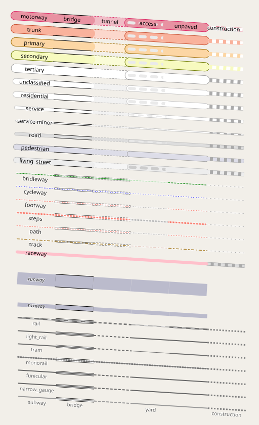
Different styling variants on all the road classes – many of these can be cross-combined
Beyond that the main principal technical disadvantages of the OSM-Carto road rendering system are:
- It requires quite a lot of SQL code being duplicated into the different road layers, in particular the tagging interpretation that is being done on SQL level. Some of this has been reduced more recently using YAML node anchors and references – specifically the roads-casing and roads-fill layers as well as the turning-circle-casing and turning-circle-fill layers. That only works when the SQL code is exactly identical though.
- This of course also means that it requires unnecessarily querying the same data several times from the database. Practically this is not a big issue performance wise but still it is not a very elegant way to do this.
- Any non-trivial improvements and extensions to be made to the road rendering system typically require additional layers or at least adding to the SQL code that then needs to get synchronized across several layers and adding to the already significant complexity of the whole system.
- If you look at roads.mss you can find a lot of fairly mechanical repetitions of code to implement the variation of styling parameters across zoom levels. Like the following:
[zoom >= 13] { line-width: @secondary-width-z13; }

[zoom >= 14] { line-width: @secondary-width-z14; }

[zoom >= 15] { line-width: @secondary-width-z15; }

[zoom >= 16] { line-width: @secondary-width-z16; }

[zoom >= 17] { line-width: @secondary-width-z17; }

[zoom >= 18] { line-width: @secondary-width-z18; }

[zoom >= 19] { line-width: @secondary-width-z19; }
Often this is even repeated for other layers or variants – like in this case with:
[zoom >= 13] { line-width: @secondary-width-z13 - 2 * @secondary-casing-width-z13; }

[zoom >= 14] { line-width: @secondary-width-z14 - 2 * @secondary-casing-width-z14; }

[zoom >= 15] { line-width: @secondary-width-z15 - 2 * @secondary-casing-width-z15; }

[zoom >= 16] { line-width: @secondary-width-z16 - 2 * @secondary-casing-width-z16; }

[zoom >= 17] { line-width: @secondary-width-z17 - 2 * @secondary-casing-width-z17; }

[zoom >= 18] { line-width: @secondary-width-z18 - 2 * @secondary-casing-width-z18; }

[zoom >= 19] { line-width: @secondary-width-z19 - 2 * @secondary-casing-width-z19; }
[zoom >= 13] { line-width: @secondary-width-z13 - 2 * @major-bridge-casing-width-z13; }
[zoom >= 14] { line-width: @secondary-width-z14 - 2 * @major-bridge-casing-width-z14; }
[zoom >= 15] { line-width: @secondary-width-z15 - 2 * @major-bridge-casing-width-z15; }
[zoom >= 16] { line-width: @secondary-width-z16 - 2 * @major-bridge-casing-width-z16; }
[zoom >= 17] { line-width: @secondary-width-z17 - 2 * @major-bridge-casing-width-z17; }
[zoom >= 18] { line-width: @secondary-width-z18 - 2 * @major-bridge-casing-width-z18; }
[zoom >= 19] { line-width: @secondary-width-z19 - 2 * @major-bridge-casing-width-z19; }That adds a lot of code volume and is prone to errors. It also makes styling changes that go beyond simple adjustments of the parameters in the CartoCSS symbols used complicated.
On the level of currently present functionality some of the most significant limitations of the current system are (and note these are only those related to the main road layer stack as described – things like road labeling are a different story):
For the polygon features rendered (that is primarily highway=pedestrian and highway=service polygon features) there is no support for bridges and tunnels. That means the above grid example with highway=pedestrian and highway=service polygon features looks like this:
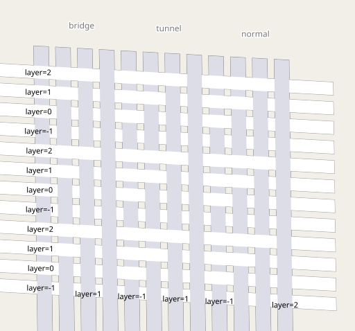
Layering of highway polygons in OSM-Carto
Solving that would be possible but you would have to integrate the polygons into all the linear road layers and that would significantly increase their complexity (and the amount of code that needs to be duplicated between them). Same applies for turning circles obviously – although this is a much less significant limitation practically of course.
Another limitation is that while the waterway bridges are correctly layered among themselves they are not interleaved with the road bridges. So a waterway bridge is always drawn below a road bridge independent of the layer tags.
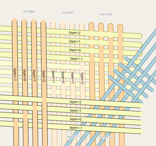
Road layering with waterway bridges in OSM-Carto
Practically this is not a big limitation of course (how many waterway bridges are there on Earth where there is a road bridge below?).
What is more important is that for avoiding complexity OSM-Carto has some features not within the road layers that should be included because they can be above or below road features in reality. Specifically that is bus guideways (which have always been separate creating various issues) and airport runways and taxiways (separated more recently) – which is rarely a problem but there are cases where it is (though in most cases of enclosed pedestrian bridges spanning taxiways the bridge is purely mapped as a building and not as a footway).
What i have not covered are the frequent concerns about overall drawing order of roads, in particular road polygons, above other map features, in particular buildings and landcover features. That is a whole other subject and one connected to much more fundamental question about map design and mapping semantics in OpenStreetMap. And it is not something related to the specific design of road layer rendering used by OSM-Carto.
Conclusions on part 1
I tried above to explain how OSM-Carto renders roads and how this system – while being one of the most sophisticated road rendering systems you can find in OSM data based maps – has its limitations. Anyone who tries to implement improvements to map rendering in the style in any way related to roads struggles with those. In the course of my work on the alternative-colors style i have now decided to try re-designing the roads rendering in a fairly fundamental way. How this looks like and what new features and improvements can be achieved with that will be subject of the second part of this post.
Pingback: weeklyOSM 567 | weekly – semanario – hebdo – 週刊 – týdeník – Wochennotiz – 주간 – tygodnik
February 2, 2022 at 16:07
I stumbled over this page trying to get railways being rendered over taxiways on my personal map.
I understand that it’s very, very complicated.
Thank u for posting your knowledge.
Carlo
February 2, 2022 at 16:10
As a matter of fact I want all highways and railways rendered over taxiways and runways.
Have a good one!
Carlo
February 10, 2023 at 19:51
Thank you so, so much for this post. I’ve been scouring the internet for an explanation of this.