
This is the second part of a two part post on roads rendering in OpenStreetMap based digital rule based map styles. In the first part i have explained and analyzed the roads rendering system of OSM-Carto and its issues, here i want to explain and discuss the re-designed road rendering system i drafted for the alternative-colors style and the improvements and new features i implemented in it.
A big warning upfront: This road rendering framework is essentially just a sketch. I will explain in the end what i hope in the long term eventually will come out of it. At the moment this is – as said – a bit sketchy and i don’t want to make any claims that it is overall better by any metric than the existing one in OSM-Carto. Or in other words: It is as much a study on what is possible as much as it is one for what is not. Keep that in mind when you think about actually using this. Also if you work with this technique or in general with the AC-style you should be sure to turn off JIT optimization in the Postgresql configuration. Because that does not deal well with the kind of queries used here apparently.
Rethinking layered rendering
The technical limitations of the OSM-Carto road rendering system i discussed in the first part are to some extent caused by specific design choices in OSM-Carto. But for the most part they are the result of principal limitations of the toolchain used by OSM-Carto. The most fundamental limitation of that is that the order in which you query the data from the database and how this is split into a lot of separate queries is directly tied to the order in which things are drawn on the map. There are some limited options to interfere with that on the raster compositioning level (OSM-Carto is using that a bit already and i use this more in the alternative-colors style – a topic for a different post) but in the end you are pretty fundamentally stuck with this paradigm of query order and drawing order being tied to each other.
Most of the software OSM-Carto is using – specifically Carto and Mapnik – are no more actively developed. That means there is not much of a chance that anything will change about this constraints. This also means that the only major component of the OSM-Carto toolchain that is still actively developed is Postgresql and PostGIS.
This essentially suggests the most promising path for rethinking the roads rendering is to work around the limitations of the layered rendering framework as described by combining all road rendering components into a single layer. If you look at the layer list in the first part with 16 layers you can see that this is a pretty radical step. Fortunately there are already quite a few pre-existing changes in the alternative-colors style that make this a bit simpler. Some layers i have dropped (tourism-boundary), others i had moved outside the road layers range (cliffs), which leaves the following layers to deal with:
- tunnels
- landuse-overlay
- line-barriers
- ferry-routes
- turning-circle-casing
- highway-area-casing
- roads-casing
- highway-area-fill
- roads-fill
- turning-circle-fill
- aerialways
- roads-low-zoom
- waterway-bridges
- bridges
In addition i moved the aerialways layer above the bridges (because practically most aerialways will probably be physically above bridges they cross) – although this could in the future be changed and integrated back with taking the layering into account of course. That is still 13 layers of course.
So why would i want to combine all of this in a single layer? This has a number of advantages. Since one layer means one SQL query only you don’t have to query stuff several times from the database and you can avoid duplication of SQL code much better. At the same time addressing some of the fundamental limitations of the OSM-Carto road rendering, in particular the lack of proper layering for highway polygons, becomes much easier and does not require a significant volume of additional code.
And most importantly you don’t have to deal with the limitations of the various methods to define the drawing order i discussed in detail in the first part and the complex and difficult to understand interaction between them because you can simply put the features in the order you want to render them in using ORDER BY in SQL. That means you cannot use group-by and attachments any more of course and for every use of attachments you have to essentially duplicate the features to be drawn in SQL (like using a UNION ALL query). But practically that is relatively simple and adding an ORDER BY statement to the wrapping query of the single roads layer is a much more intuitive and better maintainable way to do this in my opinion.
Layering in SQL
So how does the query combining all these 13 layers and the improvements i implemented look like? Before you go to looking through the more than 1700 lines of SQL code you can have a look at the basic structure where i stripped most of the actual queries, in particular the lengthy column lists which make up most of the query. A more elaborate sketch of the structure is available as well. The query makes fairly extensive use of common table expressions to query different sets of features and then use them in different contexts. On the base level of the query (roads_sublayers) we have the CTEs
roads_all– which contains all the linear road features from tunnels/bridges/roads-casing/roads-fill as well as things derived from them (for new features – i will discuss those later),road_areas_all– which contains all the road polygon features from highway-area-casing/highway-area-filltc_all– which contains the stuff from turning-circle-casing and turning-circle-fill
These CTEs currently are independent of each other. roads_all basically contains the UNION ALL from the existing road layers combining highway lines and railway lines – plus the alternative-colors specific features, which use a number of additional CTEs that reference each other.
Based on the three main CTEs there is a stack of 16 sublayer queries combined with UNION ALL. You can find the non-road layers from the above list in there while the road layers do not match the legacy layers directly. Ignoring for the moment those sublayers connected to new alternative-colors specific features we have:
casing
background
fill
area_casing
area_fill
tc_casing
tc_fill
waterway_bridges_casing
waterway_bridges_fill
line_barriers
ferry_routes
landuse_overlay
We don’t need separate sublayers for tunnels and bridges because the sublayers are not what primarily defines the drawing order. The drawing order is defined by the ORDER BY statement that follows the sublayer stack.
That means across all sublayers with a non-null int_bridge attribute (that is everything except the non-roads layers) the features with int_bridge=yes are rendered on top in the order of their layer tag. It does not matter what these are, whether road line bridges, highway polygons, turning circles or waterways. Same for tunnels at the bottom. Apart from that the ordering is similar to the one in OSM-Carto – although i made some adjustments, the effects of which are however mostly very subtle.
Map design in SQL
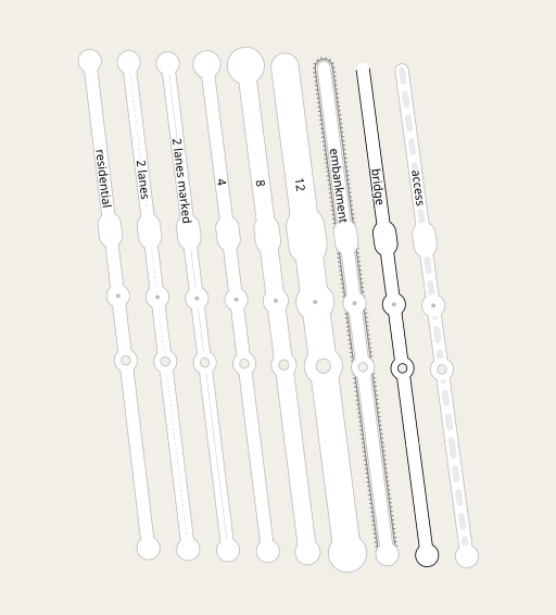
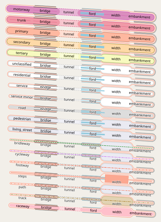
The most important result of this change is that it allows consistently layering all bridge and tunnel features – no matter if linear roads, highway polygons or waterway bridges – according to the layer attribute as explained in the first part. Here the layering in comparison between OSM-Carto and the alternative-colors style:
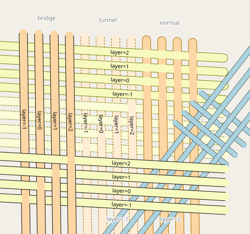
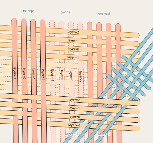
Linear roads and waterway bridges layering in OSM-Carto (left) and AC-Style (right)
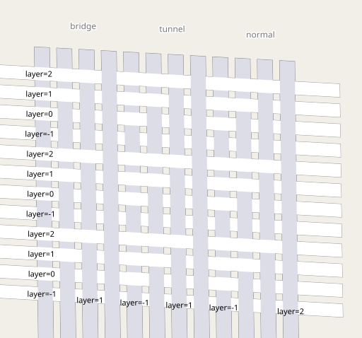
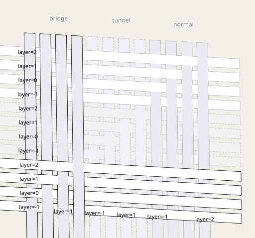
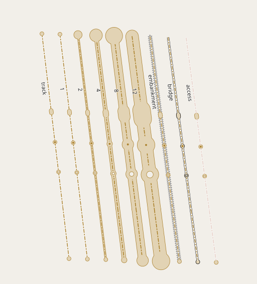
Highway polygons layering in OSM-Carto (left) and AC-Style (right)
The other fundamental thing i changed and that was also an important prerequisite for the new features i added is to define the line widths for drawing in SQL. This has a two-fold purpose: First it is to make these settings available in SQL for geometry processing and second: To avoid the error prone repetitive way of defining the drawing widths for the different zoom levels as shown in part 1. Parts of this change were already implemented in previous changes where i introduced implicit embankment rendering. This is currently based on a YAML file where you define the different line widths. This file is processed by a python script into alternatively MSS code or an SQL function containing nested CASE statements for selecting the line width based on zoom level and road type. This method is not yet set in stone – an alternative would be to have a separate table in the database containing the line width values. I have now extended approach to also include the casing width values in addition to the overall line width.
Ground unit line width rendering
One thing this change facilitates is allowing to more easily implement ground unit line width rendering at the high zoom levels. The motivation for that is the following: At the low zoom levels roads are universally rendered with a line width larger than their real physical width on the ground. That is universally the case in maps because otherwise the roads would not be visible at smaller scales and even when they would be that would not make for a well readable map. There is however a transit at some point where the drawing width or the roads becomes less than the physical width of the roads. That transit typically happens – depending on latitude, road class and the specific road – at zoom levels between 16 and 18. Drawing the roads more narrow than they are physically is however typically not of benefit for map readability and it also conflicts with the general aim you have when designing large scale maps to move to less geometric abstraction and a depiction closer to the geometric reality on the ground.
Unfortunately you cannot address this simply by increasing the nominal drawing width of the roads in general because not all individual roads of a certain class have the same width of course and what you definitely don’t want at the high zoom levels is to draw the roads wider than their actual width and then obscure other content of the map next to the roads. And fortunately quite a few of the roads in OpenStreetMap have a physical width specified – two million (or about 1 percent) and even more (12 million or 6 percent) have a lanes tag that allows estimating the likely physical width of the road with some accuracy.
To be able to draw lines in ground units on the map you have to be able to convert between map units (also called Mercator meters), ground meters and pixels on the map. The conversion factor between ground units (as tagged with the width tag for example or as estimated from the number of lanes) and map units is called the scale factor of the projection and unfortunately there is no support for directly getting that in PostGIS. I used a generic function that allows approximating that:
ST_DistanceSphere(

  ST_Transform(ST_Translate(geom, 0, 1), 4326),

  ST_Transform(geom, 4326)

)::numeric from (select ST_Centroid(!bbox!) as geom) as p
I do this based on the bounding box of the metatile – not so much for performance reasons but because that ensures geometry processing within a metatile is using the same scale factor – which is essential in some cases. At the zoom levels in question the scale factor will never vary significantly across a metatile. One thing to consider of course in the future is to – for Mercator maps – replace this generic function with the simpler formula specifically for the Mercator projection (because that function is used quite a lot).
The conversion between map units and pixels on the map by the way is the factor !scale_denominator!*0.001*0.28 – so in total you have
pixels = ground_meters/(scale_factor(!bbox!)*!scale_denominator!*0.001*0.28)
This formula is used in carto_highway_line_width_mapped() – which is implemented in roads.sql. Overall the rule for the line width of roads is as follows:
- If a width is tagged use that as the ground width.
- If no width is tagged but the number of lanes is tagged then estimate the overall ground width based on the road class and (conservatively estimated) the typical lane width for that type of road.
- If the ground width determined that way is larger than the nominal line width set by the style than draw it in that width, otherwise in the nominal width.
Currently the style still contains double drawing of the roads in both nominal and ground width (essentially determining the maximum graphically) because i initially had them rendered in different styling. But that should be removed in a future version.
Here is how this looks like at z17 with various different tagged width values – in comparison for different latitudes to show the effect of the variable scale.
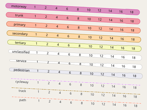
Ground unit rendering of roads at z17 at 40 degrees (left) and at 60 degrees latitude (right)
This applies for the roads drawn with the standard casing + fill style. For airport runways the formula is varied to estimate the likely width based on the runway length (using a formula initially suggested for OSM-Carto). For road features with a simple solid/dashed line signature (paths/tracks) the ground width is only visualized at z18 and above – using the styling of footway and track polygons (with some adjustment for tracks to avoid the appearance being too heavy) in addition to the centerline signature. And this ground unit visualization is only used when the drawing width in ground units is large enough to be meaningfully depicted in addition to the centerline.
The ground unit rendering of roads however is not technically as simple as it might seem because of another implicit assumption made by the roads rendering system in OSM-Carto, namely that the drawing order of road classes with the same layer as defined by z_order is in sync with the drawing width progression. That is of course no more universally the case when the tagged width is depicted which would lead to artefacts like the following.

Solving this requires modifying the road geometries in those cases which is kind of a hassle to do.

Lanes visualization
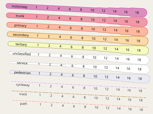
Since i already made use of the lanes tagging for estimating the ground unit width of roads i decided to visualize the number of lanes at the high zoom levels as well. As you can see this follows the implicit rules documented which say that trunk roads and motorways are assumed by default to be two lanes. lane_markings=no is indicated with dashed lines instead (click on the image to see).

Lanes visualization at z18+ (click to see also the unmarked version)
In practical use cases ground unit line width rendering and lanes visualization looks like this:


This one demonstrating the unfortunate and semantically nonsensical practice of German mappers to tag every road under a bridge as a tunnel.
Of course this style of visualization for both the lanes and the tagged width of the road does not work too well when the number of lanes and the road width changes. This requires mapping and interpretation of additional data, in particular what is mapped with placement=*, which is currently not taken into account.
Turning circles & co.
While we are on the matter of drawing width or road lines – i also extended the existing visualization of turning circles and mini-roundabouts from OSM-Carto with distinct symbolization of both of these as well as turning loops and passing places.
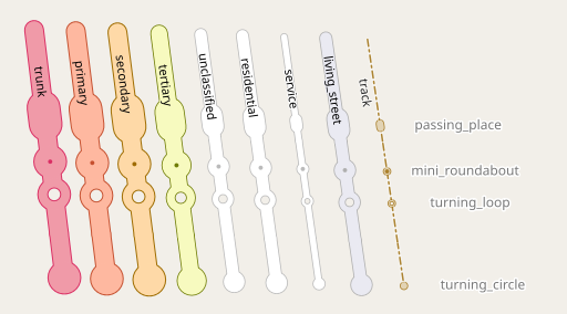
turning circles, turning loops, mini-roundabouts and passing places at z17
All of course working in combination with the bridge layering and variable width depiction. The diameter tag for turning circles is also taken into account.
turning circles etc. in combination with specified ground width or roads and tagged diameters, bridges etc. for residential roads …
… as well as tracks
Sidewalks
The next new feature i looked into visualizing is implicitly mapped sidewalks and cycle tracks. Like in case of embankments sidewalks can be mapped both implicitly as an additional tag on the road (sidewalk=both/left/right) as well as explicitly separately as a way with highway=footway and footway=sidewalk. Both are widely used and there is no clear preference among mappers and it is therefore a bit problematic that OSM-Carto only renders the explicit sidewalks. Like in case of embankments the explicit version is easier to render in a primitive fashion while good quality visualization is much easier with the implicit mapping because you can more easily take the relationship between the road and its sidewalk into account.
What i implemented is a demonstration how visualization of implicit sidewalk mapping as well as that of implicit cycleway tracks with cycleway:right=track/cycleway:left=track can work. This is shown at z18 and above

Rendering of sidewalks and cycleway tracks
and works also in combination with bridges, fords and implicit embankments. They are not rendered on tunnels to avoid obscuring ground level features.
Rendering of sidewalks in combination with various road variants
And here is how this looks like in real world situations.

Sidewalks in Ladenburg at z18

Sidewalks in Portland at z18
Steps details
Rendering of roads in their ground unit width also provides more space to visualize additional details on steps. The normal drawing width of steps does not really provide enough room for showing more information without affecting the recognizably of the steps signature. Here is what is shown with nominal drawing width and when the drawing width is large enough at z18+ for wider steps tagged with their width.
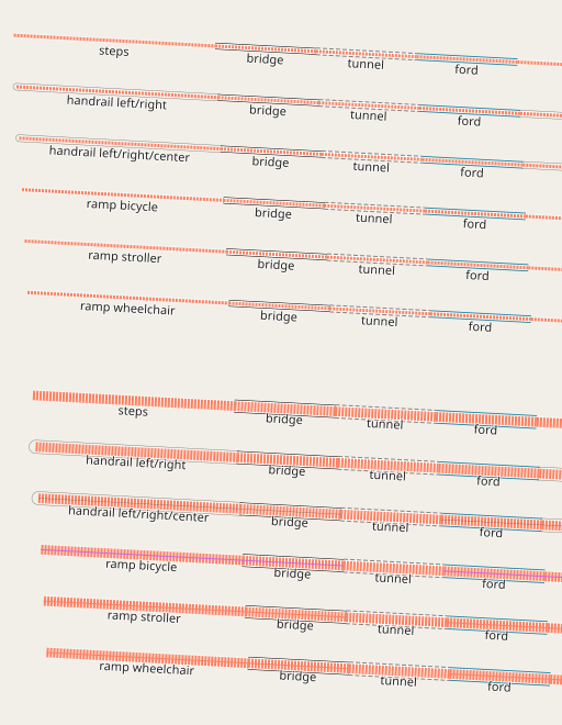
Steps details at z18+
Unpaved roads
The distinct depiction of paved and unpaved roads is one of the oldest open issues in OSM-Carto. The difficulty is that it has to work in combination with a lot of other road properties already visualized. Various forms of dashing have been tried and have been found either to be very noisy in appearance or too similar to existing depictions of tunnels (which use a dashed casing), construction roads (which use a dashed fill) or access restrictions (which use a dashed centerline on the fill) to be intuitively understandable without affecting map readability in general. The most promising idea so far has been the use of a fine grained structure pattern for the road fill. That is highly intuitive in its meaning and can be tuned to be fairly subtle. Lukas Sommer has developed this idea some time ago to be ready for use but unfortunately Mapnik did not support 2d fill patterns for line features and while this was added as a feature some time ago this is not yet available in many production environment and especially not in release versions of Kosmtik. And workarounds for this are a bit ugly to implement in the OSM-Carto road rendering system. I have now added this to the AC-style by generating polygon geometries for the unpaved roads using ST_Buffer() and rendering those instead of the normal line features. That is easily possible with the new setup since the line widths are available on SQL level anyway.

The basic styling of the unpaved road rendering used – click to see at z18 with and without tagged width visualization
It is important to consider how this looks like in combination with various other road properties – which you can see in the following illustration. There are some issues with the readability of the access restrictions – which is mostly due to their depiction offering very different levels of contrast on the different fill colors. That needs a closer look at and either tuning the access restriction color or revisiting the principal design of this feature in general.

Unpaved road styling in combination with other road attributes at z17 – click to see more
Also here a few examples of practical situations with this styling.

Unpaved roads

Unpaved pedestrian area
Open ends
That’s it for the main new road features and improvements i introduced within the new road rendering framework. There a quire a few other tweaks improving consistency in rendering – like getting tunnels and bridges rendered for raceways. And a subtle centerline on runways and taxiways. And as already hinted at there are quite a few open ends in the whole thing design wise that could use further work. But this blog post is already longer than it should be so i will close for now.
Performance of this new roads rendering approach in terms of computing resources required is not bad by the way. While the roads query is often the slowest query of the style – which is not that astonishing because it contains the data previously processed by a lot of different queries – it is not exceedingly slower than other queries. And it is often faster than the water barriers query, which has been the slowest so far and which is why i added an option to disable that for faster rendering.
Technically one important thing left unfinished is that there is currently a lot of duplication of rendering rules between SQL and MSS code. Like for example i have introduced several zoom level selectors in SQL to limit certain queries to specific zoom level ranges (of the form WHERE z(!scale_denominator!) >= 18) which are unnecessarily mirrored by a matching selector in MSS. This is redundant and prone to errors so it is important to come up with some clear principles which parts of the style logic should be in SQL and which in MSS code.
I updated the sample rendering gallery to the style changes by the way and also added quite a few new samples there.
Conclusions on part 2
The main outcome of the whole endeavor of re-designing the road rendering system this way from my perspective is that
- yes, there are much better ways to structure rendering of the roads in an OpenStreetMap based map style without taking shortcuts and as a result failing to consistently representing the road topology than the classic OSM-Carto road rendering setup.
- The ad hoc implementation of this in the way presented here based on the Carto+Mapnik toolchain is anything but ideal. In particular the difficulty of debugging the SQL code is a major concern.
- The map rendering framework that provides a decent platform for implementing the kind of rendering of roads presented here quite clearly still needs to be developed.
My main hope is that what i show here provides valuable additional insights into what exactly the key factors are to be able to develop map design in an efficient, flexible and scalable way (and scalable here is meant from the perspective of style development, not from the side of rendering efficiency – which is an important matter too of course – though pretty much a separate issue). At least to me it seems after working on this project i now have a much better idea of what the core requirements would be for a future map rendering and design system suitable for sophisticated and high quality rule based cartography with zoom level/map scale and styling specific geometry processing.
In terms of the new features implemented it is too early to draw any definitive conclusions i think. Most of them, in particular the variable width ground unit rendering and the lanes depiction i consider to be in a highly experimental state with a lot of open issues – both technically and design wise. The question of what constitutes the core of meaningful OpenStreetMap based cartography for the very high zoom levels (z19+) that goes beyond simple extrapolation of lower zoom level designs plus functioning as a POI symbol graveyard and that does not depend on mappers essentially directly hand drawing the map is still largely undiscussed.
May 29, 2021 at 01:01
Great stuff! It would be so cool to see these kind of improvements on OSM-carto. If features such as sidewalks, unpaved streets etc should become visible on the main map style, it would also boost this kind of data being recorded by a lot!
May 29, 2021 at 11:22
Thanks. Yes, i agree that it would be good and beneficial for mapper feedback to have more supplemental road features to be shown in OSM-Carto. However as i tried to explain in the text the way this is implemented here is far from ideal due to the tools used not really being designed for the kind of cartography used. It is unlikely that there will be consensus among OSM-Carto developers to adopt the kind of roads rendering framework demonstrated here and i am inclined to agree that this in the long term is probably not the way to go. What i hope this shows is that there is a need for fundamental innovation in the technical basis and tools how we do automated rule based cartography with OSM data providing a more solid, more scalable, more ergonomic and more sustainable basis for high quality cartography.
May 29, 2021 at 13:49
You mentioned somewhere that Mapnik is not maintained anymore. If it was further developed, would you say that this would be something that could open up the path to these kind of enhancements? Or would you see Mapnik as a dead end anyway?
May 29, 2021 at 15:34
Well – i am not particularly well-versed in the inner design of Mapnik so i cannot really make a proper assessment. Mapnik still is most likely the most solid general purpose renderer out there. But over the years feature creep and other things have made it probably fairly hard to maintain technically independent of economic factors. Part of the problem is that Mapnik was designed and developed to be a tool directly targeted at end users without being able to limit its feature scope by delegating stuff significantly to an abstraction layer on top (CartoCSS was used as such on the level of rendering rules later but not on the level of actual rendering)
There are some factors that limit what could be done within Mapnik – for example being tied to AGG as the graphics engine (which has not seen active development for even longer) – those are however not the issues that concern road rendering.
Keep in mind though that Mapnik is only one part of the OSM-Carto rendering toolchain, no one will want to actually design cartography directly in Mapnik these days. So if you’d want to revive Mapnik in some form you’d have to also think about the top layer of the actual map design, i.e. CartoCSS or something similar. And the problems i discuss here with the roads concern CartoCSS limitations as much as Mapnik limitations.
May 31, 2021 at 00:50
Maybe the next step… from CartoCSS to something that accomodates the high complexity a map style needs to have to cover all those special cases, would be a DSL.
I.e. a style definition that (can) in most parts be written declaratively, but can also include script-logic directly in the style.
June 7, 2021 at 20:00
If I understand correctly, the harshly worded closing sentence tells something about the motivation of these efforts. The one I like most is showing sidewalks mapped as attributes at high zoom. Could be accompanied by hiding separately mapped ones at not as high zooms.
While the question, how to populate map-space in high zoom may go undiscussed, there are answers in the works. Isn’t that what micro-mapping is supposed to provide? Kind of mapping each tomb in the graveyard individually and their stones the same. Not everybody will be happy, c.f. https://forum.openstreetmap.org/viewtopic.php?id=72552 – I too find it mind-boggling, when a winding footway in a private garden uses more nodes than a 15 story building. But the zeal will not stop short of that. Area:highway has followers, a prolific couch mapper can create 100.000 nodes in a year, QA aside.
I think, painting streets in real width can do much much of what area:highway is supposed to do. Not all of it, of course. At least it can fill the space left by surrounding buildings in cities e.g. Maybe it would make sense to add road width to nodes and extrapolate intermediate ways? So to prevent splitting, and be compatible with future automated collection, e.g. by Lidar…
June 7, 2021 at 20:38
Thanks for the comment.
I am not sure why you read the last sentence as harshly worded. What i try to express is that not much serious work and discussion exists on digital map design (or any map design fwiw) at these scale outside the domain of technical plans (which is not part of the domain of cartography really). You are right in hinting that this is not exclusively a problem of cartography but also of mapping or in other words: Also the relationship between mapping and map rendering at these scales, in particular one that produces meaningful abstraction in the data and not just has the mappers hand paint the map directly, is something still in need to be worked out. We have some existing work in that domain, in particular in the field of 3d and indoor mapping, but that is patchy in the overall domain of mapping and also not scalable in many aspects (in particular the 3d mapping).
September 17, 2021 at 00:02
Hello, Chris, I’m working on the Map Machine project, a map rendered for OpenStreetMap. I was trying to support road lanes and discovered this post with great ideas on road rendering. Here’s my first attempt to display lanes:
https://user-images.githubusercontent.com/2399987/133559451-5ecfb484-2a8a-45db-a572-abae96272aff.png
The result is pretty similar to the approach you’ve suggested. Do you mind if I use this approach in my project?
And do you mind if I try to implement your other ideas like sidewalks, fords, surfaces, etc?
Map Machine project: https://github.com/enzet/map-machine
September 17, 2021 at 09:15
Sure you can use it – the style is CC0 after all.
What is really missing at the moment – as mentioned in the post – is interpretation of placement=* to properly display changes in width and number of lanes of a road.
September 17, 2021 at 20:30
Thank you!
Yes, you’re absolutely right. I’ve started this task with the ambition to cover the entire complexity of road structure and got stuck too quickly. So I’ve decided to implement something pretty simple first, and then improve the solution step by step. The next step should be lane specifications and placement=* tag for road connections. And after that try to solve big issues with intersections.
If you’re interested in the details, there is a discussion: https://github.com/enzet/map-machine/discussions/82