What i am introducing here is something i originally wanted to work on during this autumn’s OSM hack weekend but i made some good progress on the matter during a first preparatory look at things so i decided to go ahead with it before. If anyone is interested in the matter you can none the less come by at the hack weekend of course to talk about it.
In a way this is a followup to my work from last year on low zoom waterbody rendering which so far sadly has not found much widespread application, probably because it is a fairly strange and disturbing approach for a typical digital map designer and because i never bothered to put up a real demonstration. On a technical level what i introduce here is kind of an advancement of the work on waterbody rendering but i also combine it with some design ideas i had during the last months.

low zoom waterbody rendering from last year
Landcover mapping (i understand as such here the various kinds of areas mapped in OpenStreetMap based on either their physical surface characteristics or their primary human use – forests, farmland, builtup areas etc.) is a significant part of OpenStreetMap and quite a unique selling point of the project. Things like buildings, roads and addresses – while they exist in OSM – can also be obtained from other sources in many parts of the world in fairly good quality. Alternative landcover data available from outside OSM however usually is either old and outdated, based on automatic classification of satellite data which is often unreliable and cannot differentiate many differences or represents ought to be landuse as per local authorities instead of de facto characteristics.
Many OSM based maps show landuse areas at the high zoom levels in either a plain color or using patterns. At smaller scales landcover depiction is also useful in particular to delineate urban and rural areas and to allow the map user to identify different landscapes in particular if there is no relief depiction in the map. At small scales it is usually not the specific shape of individual landcover areas that needs to be shown but the overall distribution of the different landcover types. And due to the variable scale of the mercator projection certain needs for landcover depiction occur at different zoom levels depending on where on earth you look.
Based on these needs for plain color landcover rendering you have several options as you zoom out from the higher zoom levels:
- you can drop individual landcover classes. This is what the OSM standard style does for a long time. Water areas and glaciers start at z6, forests at z8 and most other landcovers at z10. This is highly problematic because of the geographic bias inherent in these decisions and because it does not necessarily increase readability – especially if you keep the locally dominant landcover types.
- you can fade the colors (preferably in a color neutral and uniform way – not like OSM-Carto does recently) – i would say that is the cartography equivalent to give up and use tables.
- you can perform geometric generalization of some form to the landcover shapes. This is hard to do in a way that looks good, especially for the lower zoom levels and if you have a lot of different landcover classes and it is always fairly subjective and therefore inevitably quite specific to a certain map use. See the following example for a rudimentary rendering of generalized builtup areas and forests as well as waterbodies.

Example for generalized landcover data
- you can keep rendering the landcovers as on the higher zoom levels.
- you can aggregate landcover classes into a smaller set of classes and show those at the low zoom levels.
The last two options are the ones i am going to demonstrate here. These options do not really exist if you render polygons with Mapnik or similar renderers since at successively lower zoom levels you increasingly run into more problems with performance and rendering artefacts (as i discussed a year ago with respect to water area rendering). So while you can get something out of Mapnik & Co. in such situations it will not actually really be a visualization of the map data but the abstract result of an algorithm used for something different than what it is supposed to be used for.
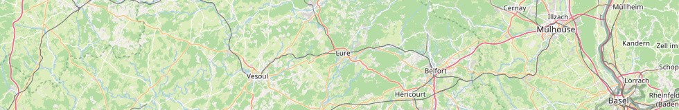
The demo i want to show here renders the landcover and water areas separately using a custom renderer and combines them with the conventionally rendered rest of the map. This is not directly possible because certain techniques used by the OSM standard style rely on the landcover layers being present. Therefore i had to do some modifications, in particular moving to preprocessed boundary data – which also allowed me to stop using Natural Earth boundaries at the lowest zoom levels and to get rid of the bogus boundaries at the 180 degree meridian.

OSM-Carto landcover and water colors alone at z9
The map shows zoom levels 1 to 9. From z10 upwards the standard style renders most of the landcovers although the current version uses the ugly color fading of course – if you want a version without the fading look at that from Geofabrik. For the alternative-colors style i currently have no higher zoom level demo.
Quite a bit could be said about the differences in the alternative-colors style but that is outside the scope here – maybe something for a future post. For the landcover it extensively implements the idea of aggregating classes as you zoom out. Here an illustration of the color aggregation scheme:

Aggregation scheme for the landcover classes
At z9 and below there are four land colors (in addition to the base land color without a mapped landcover or course) plus two glacier and three water colors. You can add to that the tidalflat color which is rendered as part of the overlay. Aggregation is of course a subjective choice and what landcover classes are included in what aggregate class is not always an easy decision. I put cemeteries into low vegetation for example although there are many cemeteries that are either largely covered with tall vegetation or vegetation free.
Since the map is rendered into separate layers you can switch on and off independently you can compare the different style variants with and without landcover rendering.

Landcover and water area layers for the alternative-colors style

With linework and labels
I also included a fallback landcover layer in the alternative-colors styling based on the Green Marble vegetation map. This of course does not completely match the definition of the aggregate landcover classes the OSM data is drawn in but it is pretty close. Where landcover mapping in OSM has gaps this layer can be used to supplement the rendering leading to globally more uniform results less dependent on the actual mapping completeness in OSM. You could interpret this as kind of a what if view for a hypothetical future perfect OSM database. Note however landcover mapping in OpenStreetMap is not based on the notion that ever square meter of the earth surface is supposed to be mapped and classified in some form – let alone that what is mapped makes sense to be rendered in a map like this.

Normal rendering exclusively based on OSM data

With fallback layer
I have not yet discussed the technical side but as said this kind of rendering cannot be produced internally with Mapnik or similar tools. The landcover and water areas are rendered using a supersampling approach which i discussed in more depth already with the waterbodies. This technique is kind of a counterpart to conventional rendering like in Mapnik – it works very well for those tasks that are prohibitively hard or impossible with Mapnik though it does not perform that well for things Mapnik is good at. The other nice thing is that the expensive part of the rendering process, producing the sample cache, is generic, i.e. independent of the actual map style with the colors and also independent of the zoom level. The two different landcover and water color schemes shown are produced from the same base rendering for all zoom levels. I have no code to publish here at the moment since the implementation is rather rudimentary without any real interface to define the styling parameters. One technical aspect i should also mention is that since the landcover data is processed with Osmium there are a number of broken geometries missing you would normally have in a rendering from an osm2pgsql database.
Regarding the demo map – ultimately this is certainly not a great map for most applications by any measure – for this it – like the OSM standard style it is based on – tries to do too many things at once. But it is meant to demonstrate approaches 4 and 5 in the list above in a solid quality implementation. My own opinion is that it beats approaches 1 and 2 hands down, especially if you view this in terms of mapper feedback and geographic neutrality but that is for the readers to decide for themselves. It certainly beats any trickery trying to implement 4 or 5 using Mapnik.
To view the demo click on any of the examples shown above and it will take you to the map with the layer configuration shown in the example. Because the map is composed from several semi-transparent layers it will be significantly slower to load than other maps of course.
December 4, 2017 at 21:05
Wow, I like the aggregation scheme. Nice work. Unfortunately right now I depend on pre-made Mapsforge maps and usually they apply tag-mapping with zoom-level limits, for e.g. residential areas appear only at Z=12 etc. so I don’t have full control with my render theme… Too bad.